Forcing
Forcing is provided via CDEPS data models documented here, in particular
This page covers forcings for the physical climate (e.g. temeperatures, winds, freshwater etc) and doesn't cover biogeochemical (BGC) forcings (dust, CO2 etc) used in configurations using the BGC model, WOMBAT.
Coupling
- DATM and DROF are coupled to the other components via the mediator - see the coupling architecture here.
- The coupled fields and remapping methods used are recorded in the mediator log output file and can be found with
grep '^ mapping' archive/output000/log/med.log; see here for how to decode this. - See the Configurations Overview page for details on how the coupling is determined.
Input data
JRA55do v1.6, replicated by NCI, is used as input data for DATM and DROF, following convention used in OMIP2 and drafted for OMIP3. For interannual-forcing (IAF) experiments, this data is available from 1958 until January 2024. For repeat-year-forcing (RYF) experiments, a single year of atmosphere and runoff data is selected (Jan-Apr 1991 and May-Dec 1990) using the make_ryf.py script in om3-scripts to generate the input files. This input data is repeated to produce the same input forcing in every model year. Stewart et al. (2020) describe the selected 12-month period to be one of the most neutral across the major climate modes of variability and less affected by the anthropogenic warming found in later years of the dataset. The paper does however remind us that the resulting model is an idealised numerical experiment and not a representation of long-term climatology.
datm.streams.xml and drof.streams.xml set individual input file paths for DATM and DROF respectively, relative to this entry in the input section of config.yaml (see the Configurations Overview page). These stream files also set time and spatial interpolation, time axes and ranges.
Atmosphere
JRA55-do atmosphere provides 3-hourly instantenous:
- sea level pressure;
- 10m wind velocity components;
- 10m specific humidity;
- 10m air temperature.
and 3-hourly averaged:
- liquid and solid precipitation;
- downwelling surface long-wave and shortwave radiation.
Input data is first interpolated to the model time within DATM, second remapped from DATM to the mediator, and lastly copied from the mediator to the ocean (MOM6) and sea ice (CICE6). The first step uses linear interpolation in time (except for downwelling shortwave, which uses "coszen" interpolation in time - cosine of the solar zenith angle). The second step remaps from the source grid (~55km resolution) to the access-om3 grid. For fluxes (precipitation and radiation), conservative remapping is applied, whilst patch remapping is used for everything else (temperature, humidity, wind). Weights for this second step are calculated during model initialisation. The third stage moves data from mediator to the ocean and sea ice model components. The mediator and active model components are on the same grid, so the only operation in the third stage is to distribute fluxes to model components by scaling fluxes using the sea ice fraction, where required. For atmosphere forcing, the landmask is applied simply as a true/false mask, as access-om3 does not have partial ocean cells. Therefore only atmosphere data over the ocean are input as forcings.
Runoff
JRA55-do runoff provides daily mean liquid and frozen runoff fields, although the runoff at many locations in the dataset is updated less frequently than daily. In the source data, all frozen run-off is distributed at the ocean surface of the Antarctic/Greenland coastlines without spreading (see issue #404).
Similar to atmospheric forcing, runoff data is first interpolated in time, second remapped from DROF to the mediator, and lastly from the mediator the the ocean (MOM6). The first and second mapping step is similar to the atmospheric forcing, namely using linear interpolation in time and conservative interpolation spatially. The last stage remapping moves from the om3 grid without a landmask to the same grid with a landmask. For liquid runoff and frozen runoff, the last stage is approached differently for each:
- For liquid runoff, the differences in landmask between the incoming data on the JRA55-do grid and the OM3 grids can cause runoff to be remapped to land cells or on cells away from the coastlines. When runoff would be placed on land cells or non-coastal ocean cells, the volume of runoff is crudely moved to the nearest coastal ocean cell using pre-generated weights from the generate_rof_weights.py script. generate_rof_weights.py selects the nearest coastal ocean cell by a BallTree algorithm using Haversine distances (i.e. the shortest disance on a sphere). The combined effect of the two remapping steps is that the full global volume of runoff enters the ocean, and only at cells which abut land cells.
- For frozen runoff, a total volume of runoff for each ice sheet is calculated and then spread according to a pattern specified in
rof2ocn_ice_spreadinnuopc.runconfig. The pattern is pre-calculated using generate_rofi_pattern.py, which regrids the source pattern (Mankoff et al., 2026)1 onto the OM3 grid. The pattern is a 12 monthly climatology and therefore changes for each calendar month. The pattern is normalised for each month in the model to ensure water conservation, so users are free to modify the pattern without impacting water conservation. There are likely to be refinements to this implementation in future releases - see #404 and #1492.
Ice surface wind stress
This is calculated in CICE6 (IcePack). The wind velocity, specific humidity, air density and potential temperature at the level height zlvl (with optionally a different height zlvs for scalars) are used to compute transfer coefficients used in formulas for the surface wind stress and turbulent heat fluxes.
The CICE6 forcing settings are in namelist group forcing_nml in cice_in. Many are unspecified and therefore take the default values.
We use the default atmbndy = 'similarity', which uses a stability-based boundary layer parameterisation based on Monin-Obukhov theory following Kauffman and Large (2002).
Because our ice-ocean coupling frequency resolves inertial oscillations we use the non-default option highfreq = .true. (Roberts et al., 2015), which uses the relative ice-atmosphere velocity to calculate the wind stress on the ice.
The exchange coefficients for momentum and scalars are determined iteratively, with a convergence tolerance atmiter_conv on ustar and maximum natmiter iterations. These take default values atmiter_conv = 0.0 and natmiter = 5. We don't use spatiotemporally variable form drag (formdrag = .false, the default).
Ocean surface stress
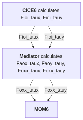
Ocean surface stress is a combination of wind stress and ice-ocean stress.
Foxx_taux and Foxx_tauy are the components of this combined surface stress received by the MOM6 cap, and are calculated in the mediator.
Foxx_taux is a weighted sum of Fioi_taux (the ice-ocean stress) and Faox_taux (the atmosphere-ocean stress), weighted by the fraction of ice and open ocean in each cell. Similarly, Foxx_tauy is a weighted sum of Fioi_tauy and Faox_tauy. The prefix Foxx denotes an ocean (o) - mediator (x) flux (F) calculated by the mediator (x). Similarly Fioi denotes an ice (i) - ocean flux calculated by the ice component, and Faox indicates an atmosphere (a) - ocean flux calculated by the mediator (see here for details on this notation).
Thus Fioi_taux is calculated in CICE6, whereas Faox_taux is calculated in the mediator (similarly for the y components).
Ice-ocean stress
The ice-ocean stress components Fioi_taux and Fioi_tauy are calculated in CICE6.
Fioi_taux and Fioi_tauy are mapped from tauxo and tauyo in the CICE6 cap, which are in turn calculated in the CICE6 cap from strocnxT_iavg and strocnyT_iavg, which are per-ice-area quantities at T points calculated from per-cell-area stresses at U points strocnxU and strocnyU.
strocnxU and strocnyU are calculated by subtroutine dyn_finish using this code; see equation (4) here and equation (2) here for an explanation. We use a turning angle \(\theta=0\) (cosw = 1.0, sinw = 0.0, the defaults), which is appropriate for an ocean component with vertical resolution sufficient to resolve the surface Ekman layer. We don't use spatiotemporally variable form drag (formdrag = .false, the default).
TODO: what namelist controls the ice-ocean stress calculation?
Atmosphere-ocean stress
The atmosphere-ocean stress components Faox_taux and Faox_tauy are calculated in the mediator.
We calculate Faox_taux and Faox_tauy using ocn_surface_flux_scheme = 0 in nuopc.runconfig, which is the default CESM1.2 scheme.
This iterates towards convergence of ustar to a relative error of less than flux_convergence = 0.01, if this can be achieved in flux_max_iteration = 5 iterations or fewer. The atmosphere-ocean stress is calculated using the relative wind, i.e. the difference between the surface wind and surface current velocity.
Surface fluxes
Salt fluxes
The net salt flux across the ocean's surface is given by the salt_flux diagnostic. Salt fluxes are associated with two different processes:
- Salt fluxes from sea ice, captured by the
salt_flux_indiagnostic in MOM6 and thefsaltdiagnostic in CICE. - Salt fluxes from sea surface salinity restoring, captured by
salt_flux_added(note that SSS restoring is applied as a salt (rather than freshwater) flux in ACCESS-OM3, because we setSRESTORE_AS_SFLUX = Truein theMOM_inputfile).
Freshwater fluxes
Freshwater fluxes with the data models (DATM and DROF) are separated in ocean, sea ice and land components as follows.
- Precipitation: precipitation over ocean and sea ice cells are scaled by the sea ice concentration in that cell. Therefore where sea ice covers part of a grid cell, a fraction of precipitation is received by each of the ocean and sea ice components, according to the sea ice concentration in that cell. Precipitation over land is discarded. Precipitation is secondly scaled such that the global freshwater going into the ocean and sea ice system is zero, see Global Freshwater Balance.
- Evaporation: evaporation (including sublimation, condensation and deposition) is calculated internally by CICE for sea ice. The mediator (CMEPS) calculates evaporation for the ocean and provides this as a surface forcing to MOM6.
- Runoff: runoff only enters the ocean. Therefore 100% of the runoff from DROF goes into MOM6.
The net freshwater flux across the ocean (MOM6) surface is given by the wfo diagnostic (sometimes the native MOM name PRCmE is used). Freshwater fluxes are associated with five different processes:
- Total precipitation, captured by the
precipdiagnostic. This is the sum of liquid precipitationlprecand frozen precipitationfprec. - Evaporation, captured by
evap. - Liquid runoff, captured by
lrunofforfriver - Frozen runoff, captured by
frunofforficeberg - Sea ice melt/formation, captured by
seaice_melt(same as the CICE diagnosticfresh)
There are also two other summarising diagnostics, net_massin and net_massout which contain the net mass of freshwater into and out of the ocean respectively. Note that these are made up of a combination of the individual fluxes described above, but that seaice_melt contributes to both depending on whether ice is formed or melted.
The net freshwater flux across the sea ice (CICE) top surface is the sum of:
- Precipitation: captured by
rain_aiandsnow_ai - Evaporation: captured by
evap_ai.
and the net freshwater flux across the sea ice - ocean interface is fresh (MOM6 diagnostic seaice_melt).
Global Freshwater Balance
For global model configurations, incoming precipitation is scaled such that the global volume of freshwater entering the ocean and sea ice total system is zero. The evaporation used in the active model components are not consistent with those used in atmosphere and runoff forcing data (JRA55do), due to different parameter choices and differences between real and modelled ocean surface conditions. Therefore a correction is applied to incoming precipitation to prevent drift in the total ocean and sea ice mass. The scaling is applied such that the global sum of runoff, precipitation and evaporation is zero. In this paragraph and diagram below: - evaporation includes evaporation, condensation, deposition and sublimation; - precipitation includes rain and snow; and - runoff includes both river and ice-sheet runoff.
---
config:
  theme: redux
  layout: fixed
---
flowchart TB
 subgraph s2["JRA55-do"]
        n1["Runoff (DROF)"]
        n6["Precipitation (DATM)"]
  end
 subgraph s3[" "]
        n2["Ocean (MOM6)"]
        n4["Sea Ice (CICE)"]
  end
 subgraph s6["Mediator - Evaporation"]
        n5["Evaporation (CMEPS and CICE)"]
        n7["Sea ice evaporation is calculated in CICE, whilst ocean evaporation is calculated in CMEPS."]
  end
 subgraph s7["Mediator - Precipitation"]
        n3["Scaled Precipitation (CMEPS)"]
        n8["Precipitation (from JRA55do) is scaled such that the global sum of runoff, precipitation and evaporation is zero at each timestep. All Runoff enters the ocean."]
  end

    n3 --> n2 & n4
    n4 --> n5
    n2 --> n5
    n6 --> n3
    n5 --> n3
    n1 --> n3

    n1@{ shape: rounded}
    n6@{ shape: rounded}
    n4@{ shape: rect}
    n7@{ shape: text}
    n3@{ shape: rounded}
    n8@{ shape: text}
    style n1 fill:#757575,color:#ffffff
    style n6 color:#ffffff,fill:#757575
    style n4 stroke:#FF6D00
    style n5 fill:#C8E6C9
    style n3 fill:#C8E6C9
    linkStyle 0 stroke:#00C853,fill:none
    linkStyle 1 stroke:#00C853,fill:none
    linkStyle 2 stroke:#FF6D00,fill:none
    linkStyle 3 stroke:#00C853,fill:none
    linkStyle 5 stroke:#00C853,fill:none
The scaling is implemented by including med_phases_scalefreshwater_run in
nuopc.runseq and setting the MOM6 option ADJUST_NET_FRESH_WATER_TO_ZERO to False.
Note, the scaling approach does not achieve exactly zero freshwater at each timestep and there is a small variation in global ocean mass (annual variation of approximately ±1e-6%). This appears to be related to CICE treatment of freshwater fluxes. Sea ice evaporation is calculated during the sea ice timestep, so is different to the evaporation used when balancing the global freshwater fluxes which is completed before the sea ice is run. In addition, precipitation is added to sea ice during the sea ice timestep, and therefore the area of sea ice to catch precipitation has changed slightly since the balancing.
Heat fluxes
Heat fluxes with the data models (DATM and DROF) are seperated in ocean, sea ice and land components as follows.
- Radiation: incoming shortwave from the atmosphere, over ocean and sea ice cells, are scaled by the sea ice concentration in that cell. Therefore where sea ice covers part of a grid cell, a fraction of shortwave is received by each of the ocean and sea ice components, according to the sea ice concentration in that cell. A small fraction of incomings shortwave penetrates through sea ice to enter the ocean.
- Sensible Heat : Sensible heat fluxes are calculated internally by CICE for sea ice. The mediator (CMEPS) calculates these for the ocean and provides this as a surface forcing to MOM6.
- Latent Heat (Evaporation): Latent heat due to evaporation are calculated internally by CICE for sea ice. The mediator (CMEPS) calculates these for the ocean and provides this as a surface forcing to MOM6.
- Latent Heat (Melt): The latent heat to melt frozen runoff (i.e. icebergs) is calculated internally in MOM6.
- Heat from mass transfer: The enthalpy transferred in/out of the ocean due to freshwater transfer is calculated in the mediator (CMEPS) and provided as a surface forcing to MOM6. For CICE6, this enthalpy flux is calculated internally.
- Precipitation and Runoff: Heat fluxes associated with transfer of freshwater are calculated in the relevant model components, for both MOM6 and CICE, based on the freshwater received by that component.
There is no prognostic process to raise/lower the temperature of freshwater fluxes to the ocean / sea ice temperature. It is assumed to enter the model at the temperature of the surrounding ocean / sea ice. There is also no process (currently) to account for latent heat to melt liquid runoff from icesheets (i.e. basal melt) - see 1197 for details.
The net heat flux across the ocean's surface is given by the hfds diagnostic (or native MOM name net_heat_surface). Heat fluxes are associated to eight different processes:
- Shortwave radiation, captured by
rsntds(or native MOM nameSW) - Longwave radiation, captured by
rlntds(or native MOM nameLW) - Latent heat, captured by
hflso(or native MOM namelatent). This is the sum of latent heat from evaporationlatent_evap, latent heat from frozen precipitationhfsnthermds(or native MOM namelatent_fprec_diag), latent heat from frozen runoffhfibthermds(or native MOM namelatent_frunoff) and latent heat from frozen runoff from glacierslatent_frunoff_glc(which is zero in ACCESS-OM3, since we don't couple to an active ice sheet model). - Sensible heat, captured by
hfsso(or native MOM namesensible) - Heat from melt/freezing of sea ice, captured by
seaice_melt_heat(same as CICE diagnosticfhocn_ai) - Heat from frazil formation, captured by
hfsifrazil(or native MOM namefrazil) - Heat from mass transfer, frozen or liquid, given by
heat_content_surfwater, which can be further partitioned into:heat_content_evap, from evaporationhfrainds, from liquid and frozen precipitation and condensation, further split intoheat_content_lprec,heat_content_fprecandheat_content_condhfrunoffdsfrom liquid and frozen runoff, further split intoheat_content_lrunoff,heat_content_frunoff,heat_content_lrunoff_glcandheat_content_frunoff_glc(again, the_glccomponents are zero in ACCESS-OM3)
- Heat from flux adjustments, captured by
heat_added(zero in ACCESS-OM3).
Note that the diagnostic net_heat_coupler includes processes 1. to 5., but not 6., 7. or 8.
References
K.D. Stewart, W.M. Kim, S. Urakawa, A.McC. Hogg, S. Yeager, H. Tsujino, H. Nakano, A.E. Kiss, G. Danabasoglu, JRA55-do-based repeat year forcing datasets for driving ocean–sea-ice models, Ocean Modelling, Volume 147, 2020, https://doi.org/10.1016/j.ocemod.2019.101557.
-
Mankoff, K., Jourdain, N., Marson, J., Olivé Abelló, A., Pierre, M., Davison, B., & Schmidt, G. A. (2026). Freshwater sources from antarctica and greenland [Dataset]. Zenodo. https://doi.org/10.5281/zenodo.14020895 ↩